


One of the most impressive and unique abilities of Grasshopper is its ability to create organically designed vases or lampshades. For this project, I loosely followed a youtube tutorial, but the work done in it is generalizable to countless projects. I’ve taken it upon myself to simplify the project for the purposes of boiling it down to only the concepts. In other words, the goal of this tutorial is only to give folks a general understanding, not to aid in the creation of something very useful. To start, we’re going to bring in 3 blocks: they are “range,” “graph mapper,” and “point cylindrical.” In order to get these blocks, double click on the canvas to open the search bar and type in the name of the block you want.
Let’s talk about what these 3 blocks do before we do anything else. The goal of the “range” block is to create a list of evenly spaced numbers between a maximum and minimum value. The “graph mapper” block allows us to provide inputs (x-values) and returns us outputs (y-values) based on the type of graph we select. Finally, we have “point cylindrical;” this hearkens back to precalculus, when we would graph points in cylindrical coordinates. This block takes a radius, elevation, and angle represented with “R,” “E,” and “A,” respectively.
1.
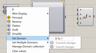
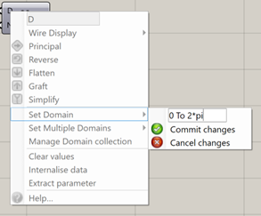
Now, let’s familiarize ourselves a bit with the software we’ll be using. Before doing anything else, consider checking out my previous blog post about the wonders of Grasshopper, and why we’re using it in this tutorial. One of the most important parts of Grasshopper is understanding that a lot of information is hidden beneath the surface, and we need to right click to uncover these options. When we right click on an input, we’re given the option of setting a value manually. This allows us to keep our canvas much cleaner. In this screenshot, I’ve right clicked my domain input on my range block and set it to “0 To 1”, which will serve as the lower and upper bound on my range block.
2.
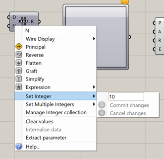
By right clicking on“N,” I find that I can set an integer value for the number of divisions. So,given these settings, the range block will cut up 0 to 1 in 10 slices.
3.
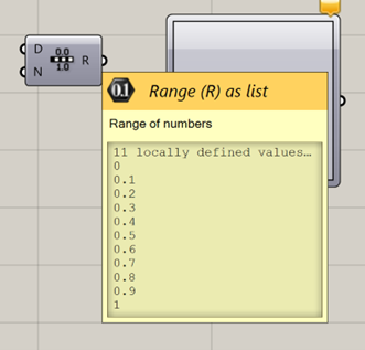
When we hover our mouse over “R”, we see the output range of 11 values from 0 to 1. This gets a little confusing because we run into issues regarding our methods of counting. Do we start at 0 or 1? Mousing over this output makes it clear that we have started counting at 1 and therefore have 11 values listed. That also makes intuitive sense, because “N” represents the number of slices, where having 1 slice gives you two values.
4.
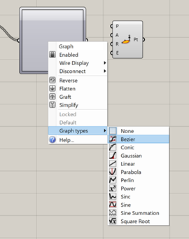
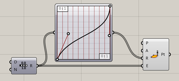
When we grab the node at the end of our range function and drag it to the graph mapper, it “wires” the output to the input. In the case of our range and graph mapper, we wire a list of values spanning from 0 to 1 to our graph mapper for input values. Once you do this, you’ll see nothing has changed. That’s because we have yet to set a graph type on the graph mapper. You may be able to guess that in order to do this, we have to right click on the graph mapper and select a graph type. Let’s use Bezier. A Bezier curve (I’ve linked the wikipedia page, but use caution… STEM wikipedia is quite scary) allows users to set the value and tangency of end points, then uses those inputs to figure out a way to graph that.
5.
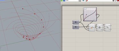
When we wire the output of our graph mapper to the input of our radius in our cylindrical points and the output of our range to the input of our elevation in cylindrical points, we get our points graphed in 2D space in the XZ plane.
6.
Now we’re going to add rotation. Let’s make a range from 0 to 2Pi so that we can do one full rotation throughout the curve’s journey.
7.
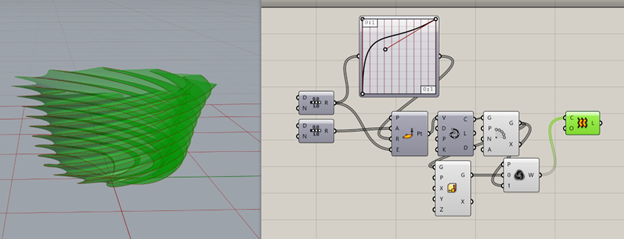
We’ll wire this to “A” on our cylindrical point to make it set the angle for each point as an evenly spaced amount. Then, we use an “interpolate” block to fit a curve to these points (mind you this is “interpolate,” not “interpolate date/a”). Wire the output of our point cylindrical to “V” or vertices on the interpolate block. We can wire this output curve to a polar array block’s “G” or geometry input. This creates a sort of coriolis of curves. Very fun!
8.
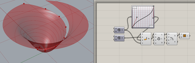
Now we’re going to turn these curves into a shape using the loft tool. Bring in a loft block and wire “G” output from the polar array to “C” or curve input on the loft. The loft tool tries to create a surface that conforms to all of the curves it’s given.
9.
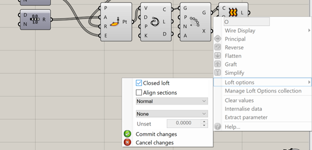
You may have noticed that there’s a huge slice missing from our loft. That’ll be a problem, so let’s fix it. To make a loft cyclic or “closed,” right click the “O” or options on the loft block and select loft options. Check the closed loft box. Then hit “commit changes."
10.
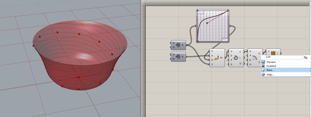
There you go! You’ve made your first lamp shade in Grasshopper! In order to actually export this if we wanted to 3D print it, we have to go through a process called baking. Baking cements our model and makes it a reality and not just a hologram in Rhino. To do this, right click the loft and select “bake."
11.
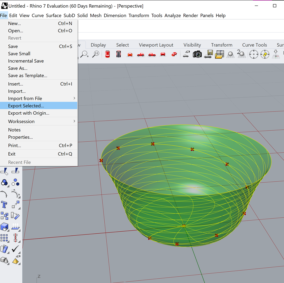
Now if we wanted to, we can 3D print the object by selecting it with left click and clicking file ->“export selected.” I will note, however, that 3D printing this object with normal settings will encounter some issues. Because we only have a surface, this print would be best printed in “vase mode,” also known by Cura as “spiralize outer contour.” This mode prints objects with a wall thickness equal to one pass of the extruder and creates a continuous path all the way up the piece. These prints are frequently less “layer-y” than ones done using traditional methods. I encourage you to play around with it!
12.
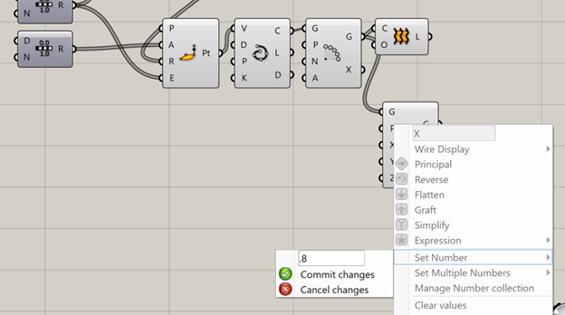
Now, if you were paying really close attention, you will have noticed that adding a spiral to the curves we made the loft from actually had no effect. Try it yourself! Delete the do this? Well, now things get a little complicated. If you felt overwhelmed by the first half of this tutorial, consider doing a few more basic things and exploring the software a little more deeply before continuing. Okay, disclaimers over. The reason I added a spiral to the curves was to lay the foundation for the creation of a “wave” effect on the surface of the shade. To accomplish this, we will use a non-uniform scale tool (Scale NU). This block allows us to change the scale of an object in independent directions. Let’s wire this to our polar array’s output geometry. Nothing happened? Well, that’s because the scaling factors are all set to 1. Let’s try 0.8 for X and Y.
13.
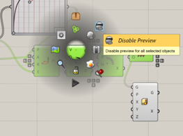
At this point, our workspace is getting pretty busy. Let’s clean it up. Select a few blocks and middle click to select “Disable Preview.” Except I’ll be keeping the polar array preview on to compare the two spirals.
14.
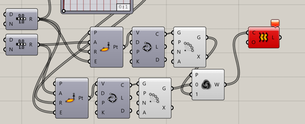
Next, we need a “weave” block. The weave tool takes two lists and weaves them into one list using a pattern. The default is 01, which is to say “item from list 0”, then “item from list 1.” Wiring this output to our loft and turning the preview back on yields this radical spiral pattern on the surface of our vase. Now this is all fine and good, but there’s an issue. This piece could never be 3D printed. It has almost perfectly horizontal overhangs. 3D printers hate any angle greater than 45 degrees, and we would be trying to feed it a 90 degree angle? It would surely fail. How can we fix this?
15.
Unfortunately, the solution to this is not an easy one. This issue arises from the fact that our curves that we are weaving are perfectly in line with each other, and we can fix this by offsetting the curves by a slight angle. So, we’re going to recreate our “0” list. Start by copying and pasting the 3 blocks we used to create the curves and replace the Scale NU with them.
16.
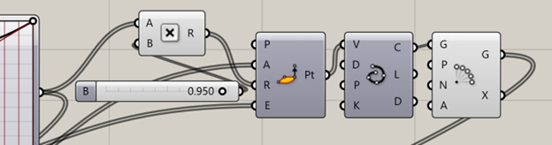
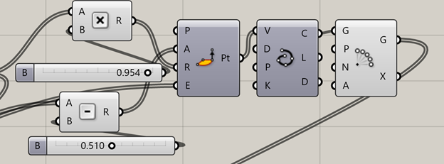
Instead of a non uniform scale, we’re going to scale our radius using a multiply block. Hooked up to one of the most powerful blocks in Grasshopper—a slider. Sliders are one of the most basic parameter blocks that empower designers to change their design in an instant. Using a multiply block, we can wire the output of our graph mapper to be multiplied by a slider value that we can adjust by clicking and dragging. Then we can wire this output to the radius of our cylindrical point plotter. Now play around with the slider and see how it changes your model. Try to get an intuitive sense for how the model is changing and why it’s changing that way.
17.
However awesome that might be, we still haven’t quite fixed our issues with the rotation of the weave. In order to do that, we’re going to add a fixed amount to the angle. So let’s start by wiring our 0 to 2pi range to a subtraction block and hooking the other end up to a slider.
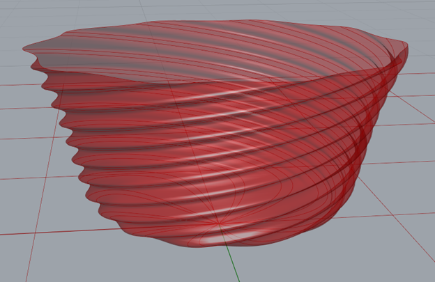
Complete!
Now play around with your sliders to change your model until you feel that you’ve gotten a wavy pattern that you like, bake your object, and get printing! Here’s mine.
Project Examples
Have a solution to this challenge you want to share? Take a photo or video of your prototype, post it on social media, and don’t forget to tag us @fluxspace_io


